After enjoying the galleries of maps published during the last year’s challenges, I decided to publish my own in 2025. You can find the instructions here.
I decided to focus on mapping with R as much as possible. The results will be uploaded to Mastodon and LinkedIn.
Enjoy them!
Day 1 – Points
Challenge Classic: Map with point data (e.g., individual locations, points of interest, clusters). Focus on effective symbolization and density visualization.
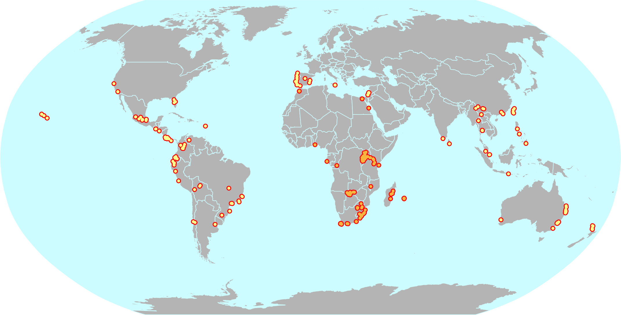
Occurrences of papyrus (Cyperus papyrus L.) worldwide according to GBIF. Orange dots are the occurrences in Africa (its natural range). Yellow dots are the occurrences outside of Africa (introduced range). The map uses the Robinson projection.
Day 2 – Lines
Challenge Classic: Map linear features (e.g., roads, rivers, migration paths, flow lines). Explore line thickness, color, and direction to convey information.
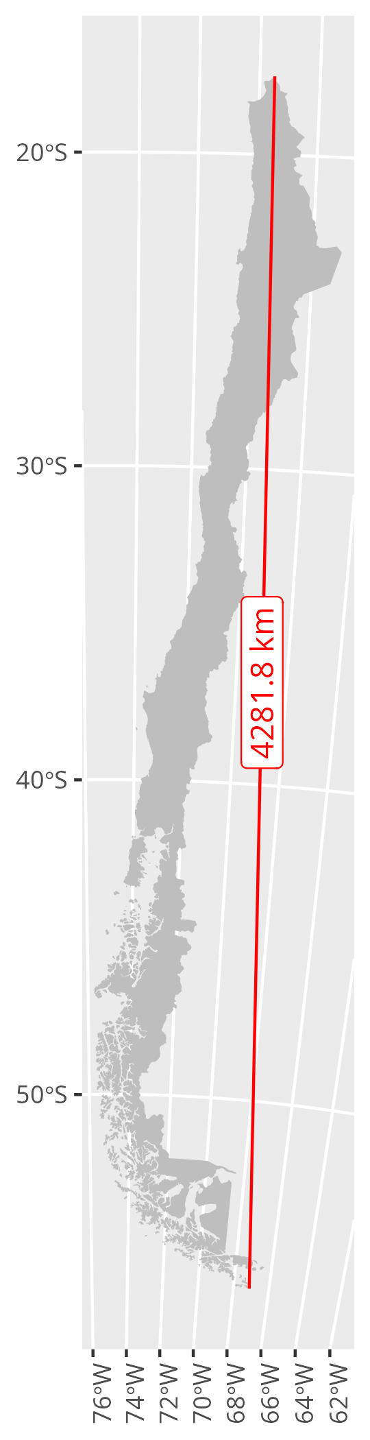
Just one line displaying the longest span for continental Chile.
Day 3 – Polygons
Challenge Classic: Create a map focused on area features (e.g., administrative regions, land use, boundaries). Use fills, patterns, and choropleth techniques.
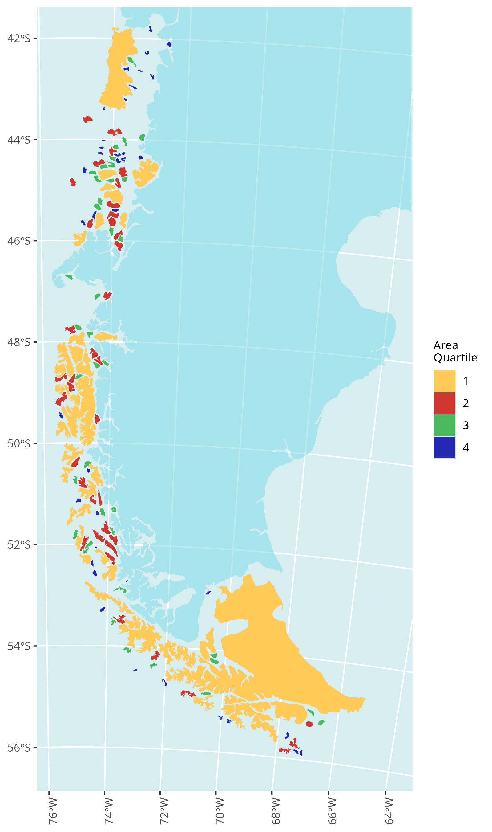
The islands of the Magellanic fjords are classified into quartiles according to their surface area.
Day 4 – My Data
Map something personal using your own dataset. Visualize GPS traces, your commute, or a unique, small dataset you created. (Need simple data? Try geojson.io).
The background is from OpenStreetMap, masked with a dark layer, and scratched by the locations of track points collected over several years.
Day 5 – Earth
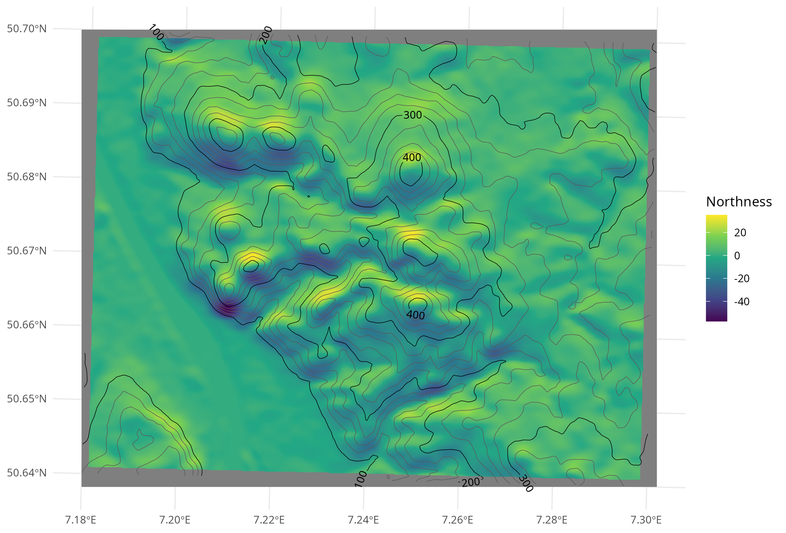
Classical Elements 1/4: Focus on the tangible and grounded. Map landforms, geology, soil, agriculture, elevation, or anything solid beneath your feet.
Northness estimated by the difference in mean elevation towards south minus towards north. The location is the Siebengebirge in Germany. Contour lines show the elevation in m asl.
Day 6 – Dimensions
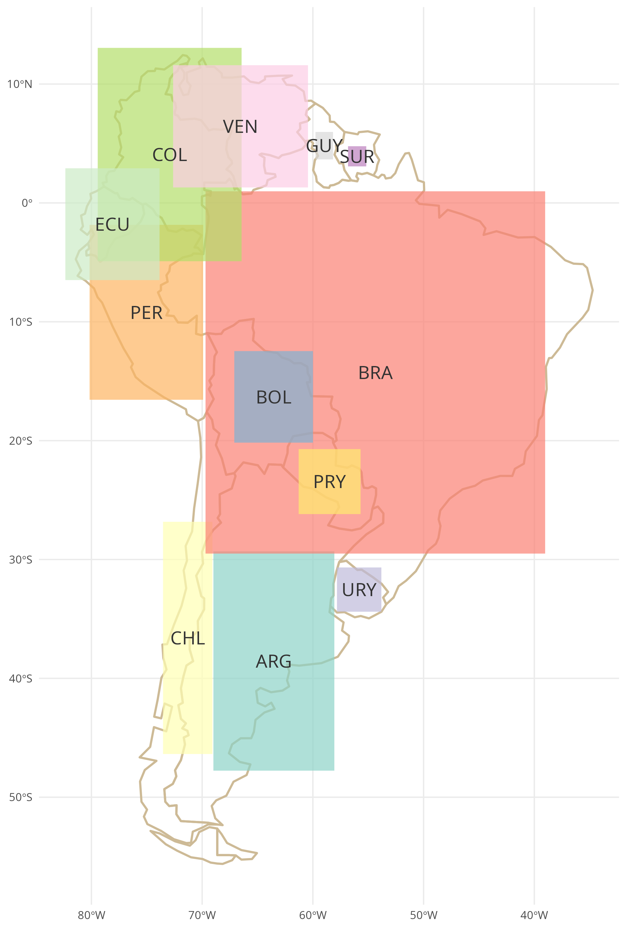
Map beyond 2D. Visualize data using 3D models, extrusions (building heights), depth, time (as a dimension), or an unconventional multivariate approach.
The population size of the South American countries is represented by the area of the rectangles. The centroid and aspect ratio of each rectangle are preserved from the bounding boxes of the respective polygons in the background.
Day 8 – Urban
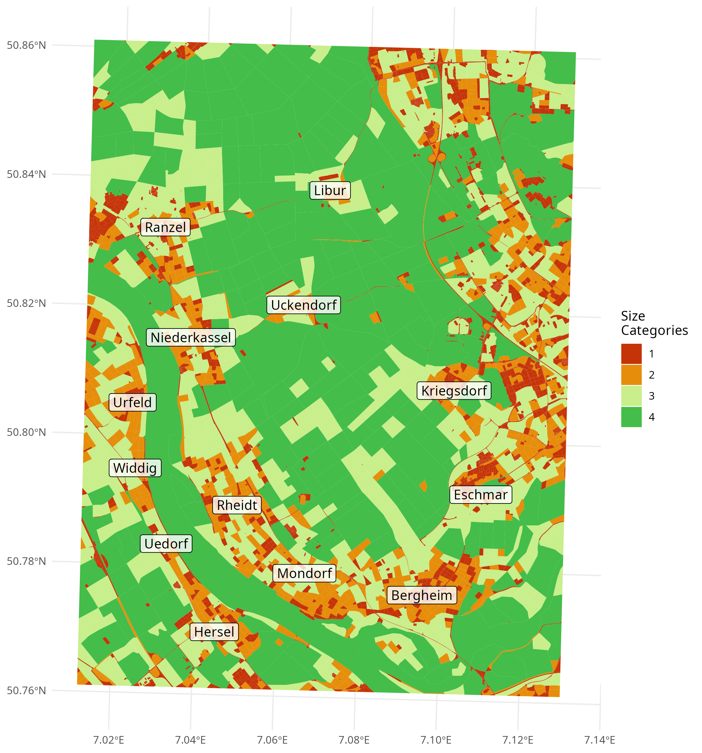
(World Urbanism Day) Map the built environment: dense street networks, highrises, urban sprawl, city infrastructure, or population density within a metro area.
The area is divided into blocks using the highway feature from OpenStreetMap. Blocks are classified primarily by size. Small blocks are expected to indicate urban areas.
Day 9 – Analog
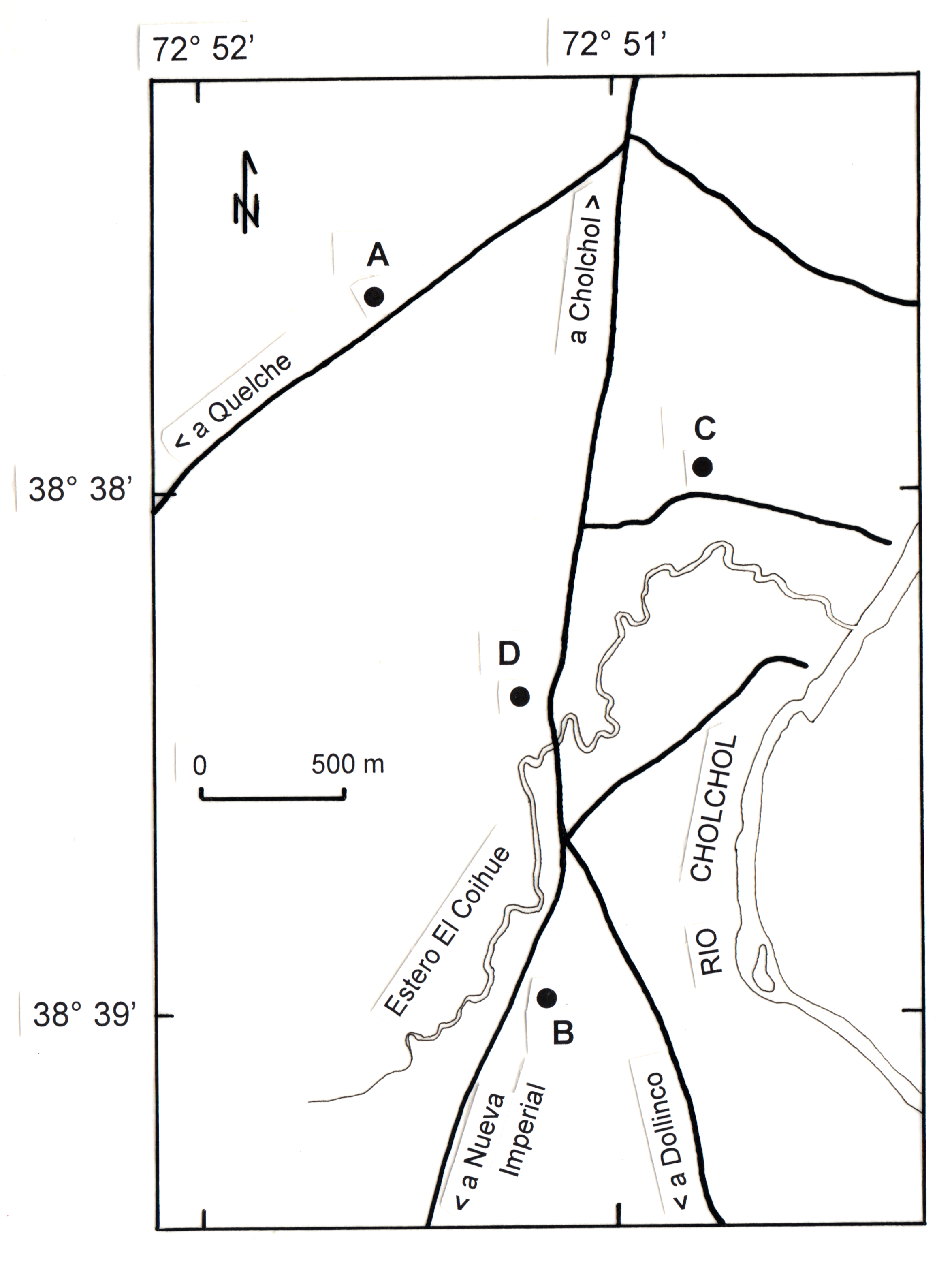
Step away from the screen! Create your map using traditional methods (e.g., pen, pencil, paint, collage, physical models). Show the handmade process!
I used to prepare maps by hand, using ink and printed labels, for our scientific publications at the Geobotanical Lab in Valdivia. The map shown here was prepared for my PhD thesis and depicts sample locations (points A to D) south of the city of Cholchol (Araucanía, Chile). The post-scan processing steps are omitted here.
Day 11 – Minimal Map
Challenge yourself to use the fewest possible elements (color, line weight, labels) while keeping the map clear, useful, and informative.
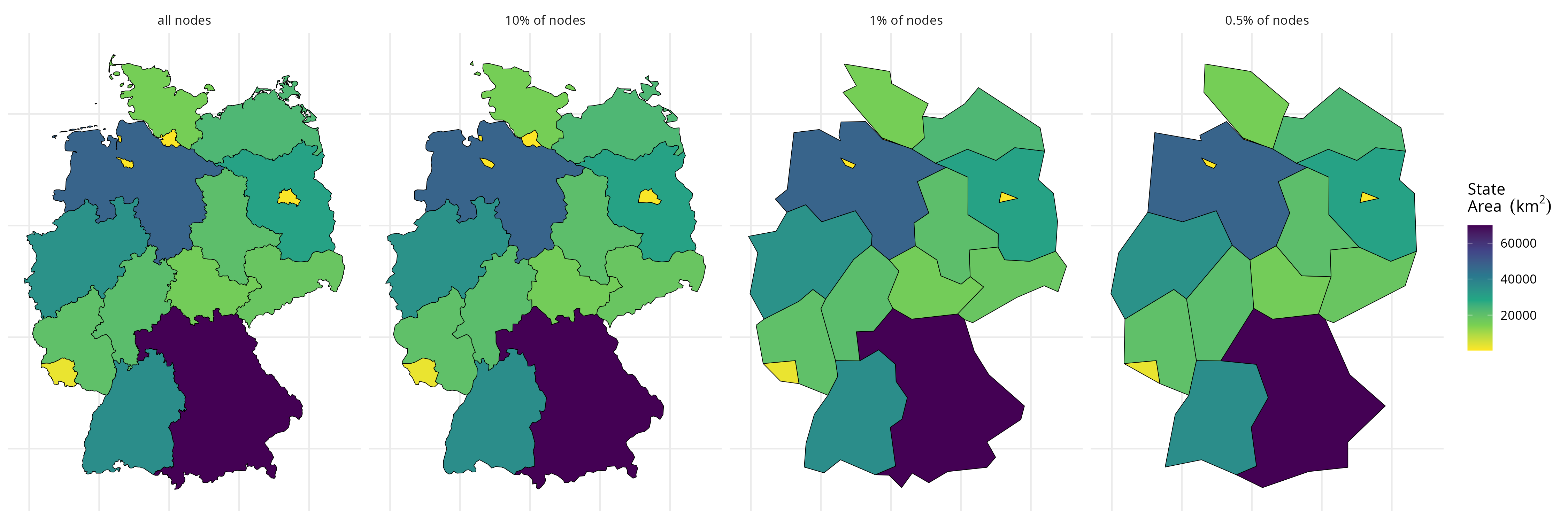
While working as a cartographer, I learned about various techniques for generalizing features on maps. Here, I applied the Douglas–Peucker algorithm (R package rmapshaper) to reduce the number of nodes. Note that this article recommends Visvalingam as an alternative. The choropleth shows the area size of the German states, calculated using the original polygons (I was too lazy to find the population data).
Day 12 – Map from 2125
How will maps look 100 years from now? Create a speculative map of what might be (or what you hope will be).
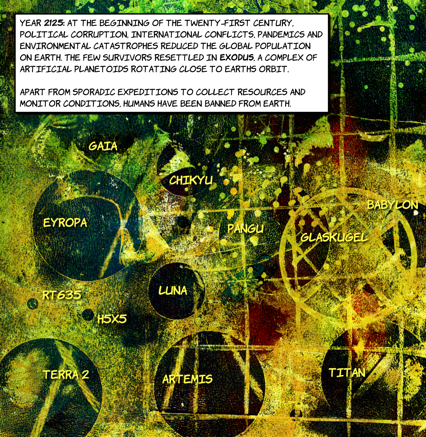
I gave an artistic piece of work (a Gelli plate print) a futuristic look for a kind of worst-case scenario.
Day 13 – 10 minute map
Start the timer! The maximum allowed time to design and produce this map is 10 minutes. Focus on speed, simplicity, and core communication.
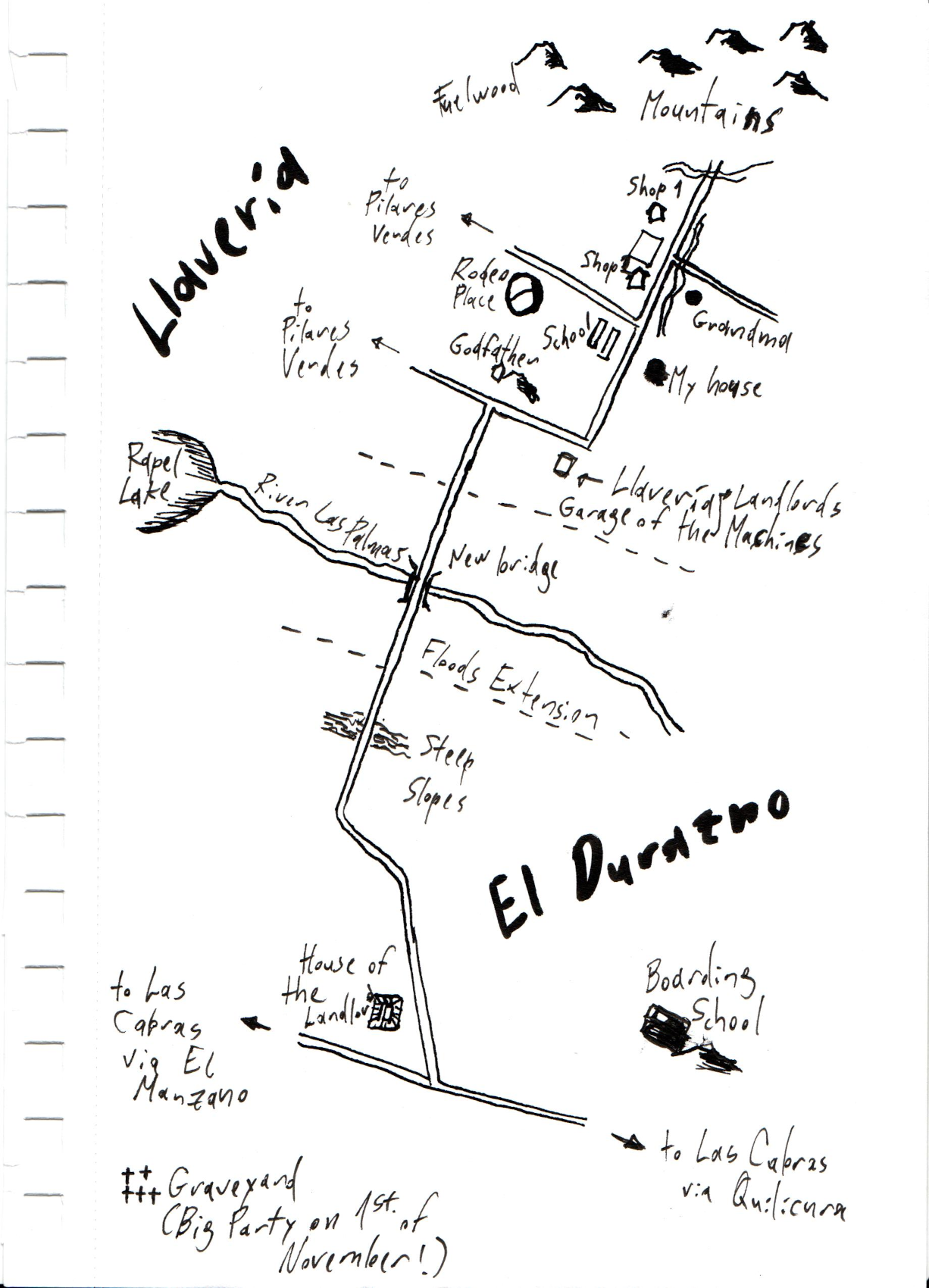
This is a personal map showing important places from my childhood in the countryside. The Llavería got its name from the old farm equipment storage buildings (llaves means “keys” in Spanish). Until the Chilean land reform of the 1960s, the place was a large estate managed according to medieval standards. In 1985, a powerful earthquake destroyed most of the remaining structures from that period, including the Llavería.
Day 14 – Data challenge: OpenStreetMap
Use OpenStreetMap (OSM) data as your primary source. Map your favorite feature, contribute back to the project, or style the map in an interesting way.
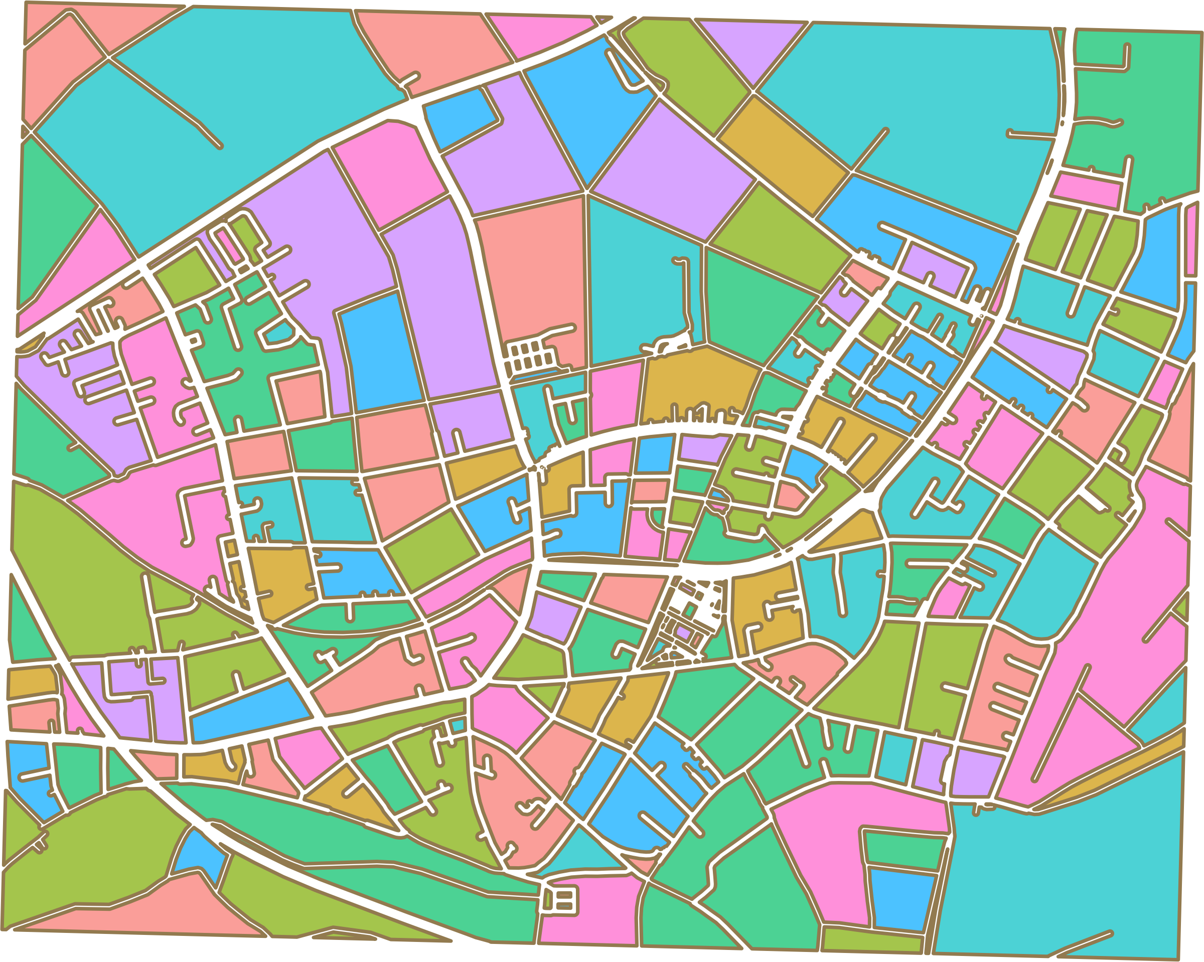
I am attempting an artistic display of road networks by using buffers according to road categories and assigning random colors to the polygons between roads. The area includes Bergheim and Müllekoven (Troisdorf), where I currently live.
Day 16 – Cell
Map something composed of small, discrete units or networks. This could be a geographic cell (raster, tessellation), a cellular network, or a biological/social process (e.g., disease spread).
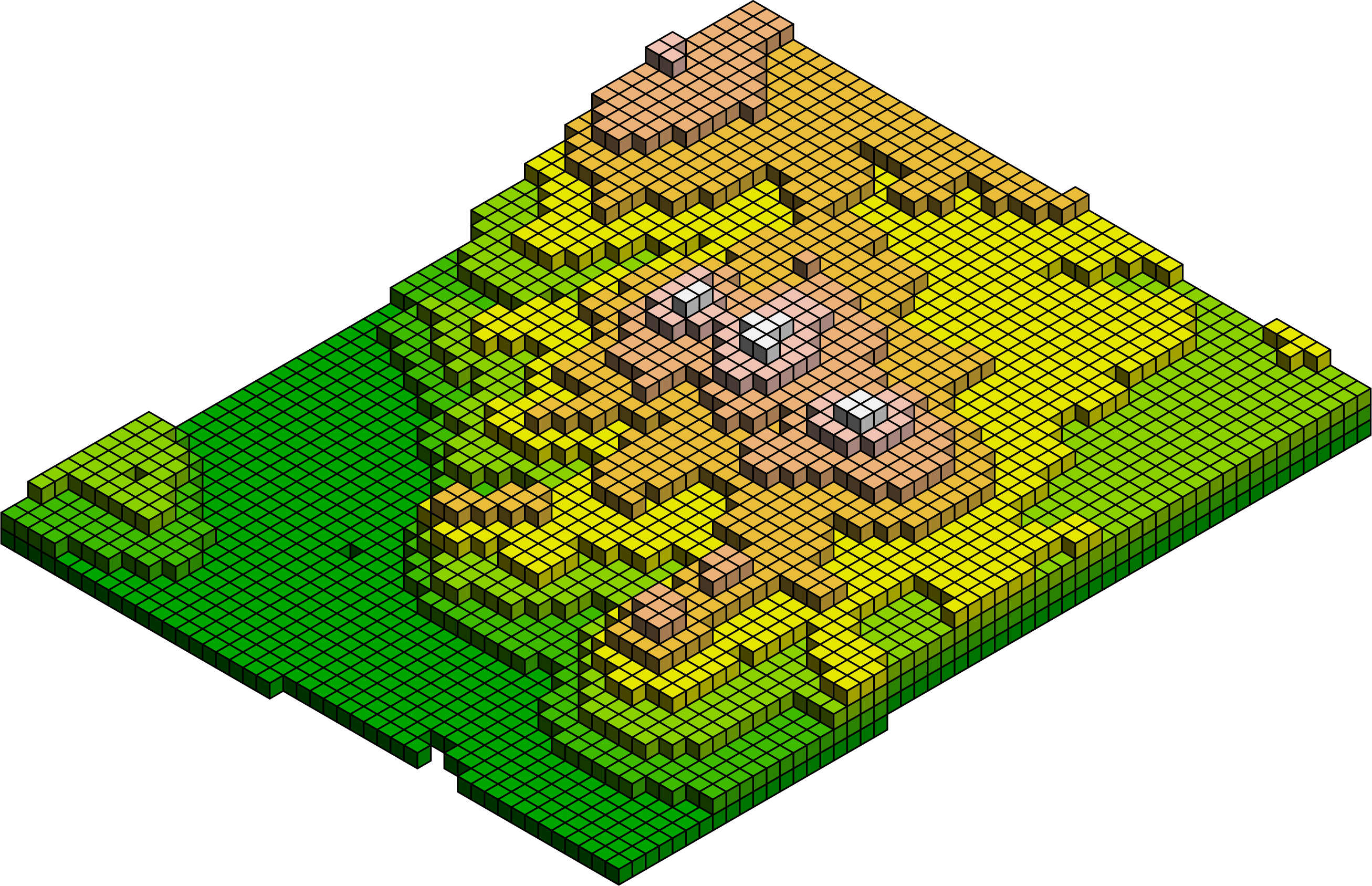
The elevation model was constructed with isocubes. The model represents the Siebengebirge in Germany (see this map). Each cube has a surface area of 150 meters by 150 meters, and the height represents an elevation of 50 meters.
Day 19 – Projections
(GIS Day) Focus entirely on map projections. Choose an unusual or misunderstood projection to highlight a theme, or visualize distortion. (See xkcd.com/977)
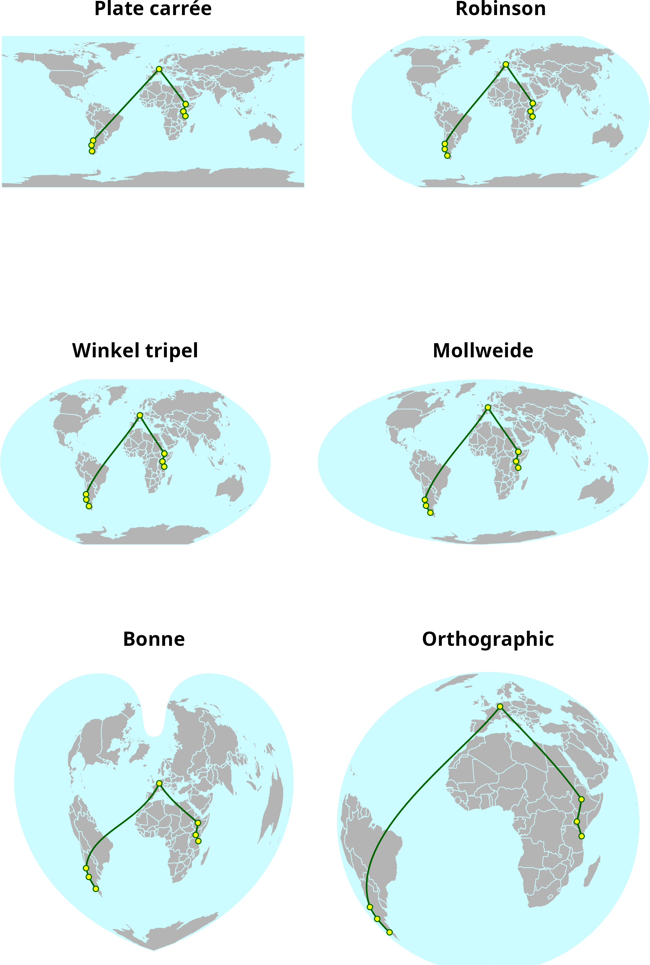
A line connecting the most important stations of my life around the world, displayed in six different projections.
Day 22 – Data challenge: Natural Earth
Use the Natural Earth dataset as your primary source for a visually stunning small-scale world or continent map.
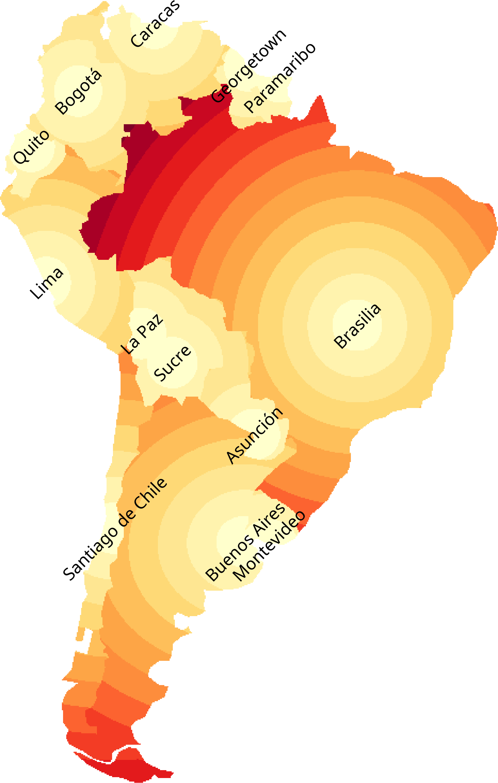
The distance to the capital cities within their respective countries. The polygons and capital cities were extracted from the Natural Earth database. Distances are classified into 250 km intervals.
Day 23 – Process
Show how you make a map. This could be a tutorial, a step-by-step graphic, a blog post, a video, or a screenshot of your work environment. Combine it with a map from another day!
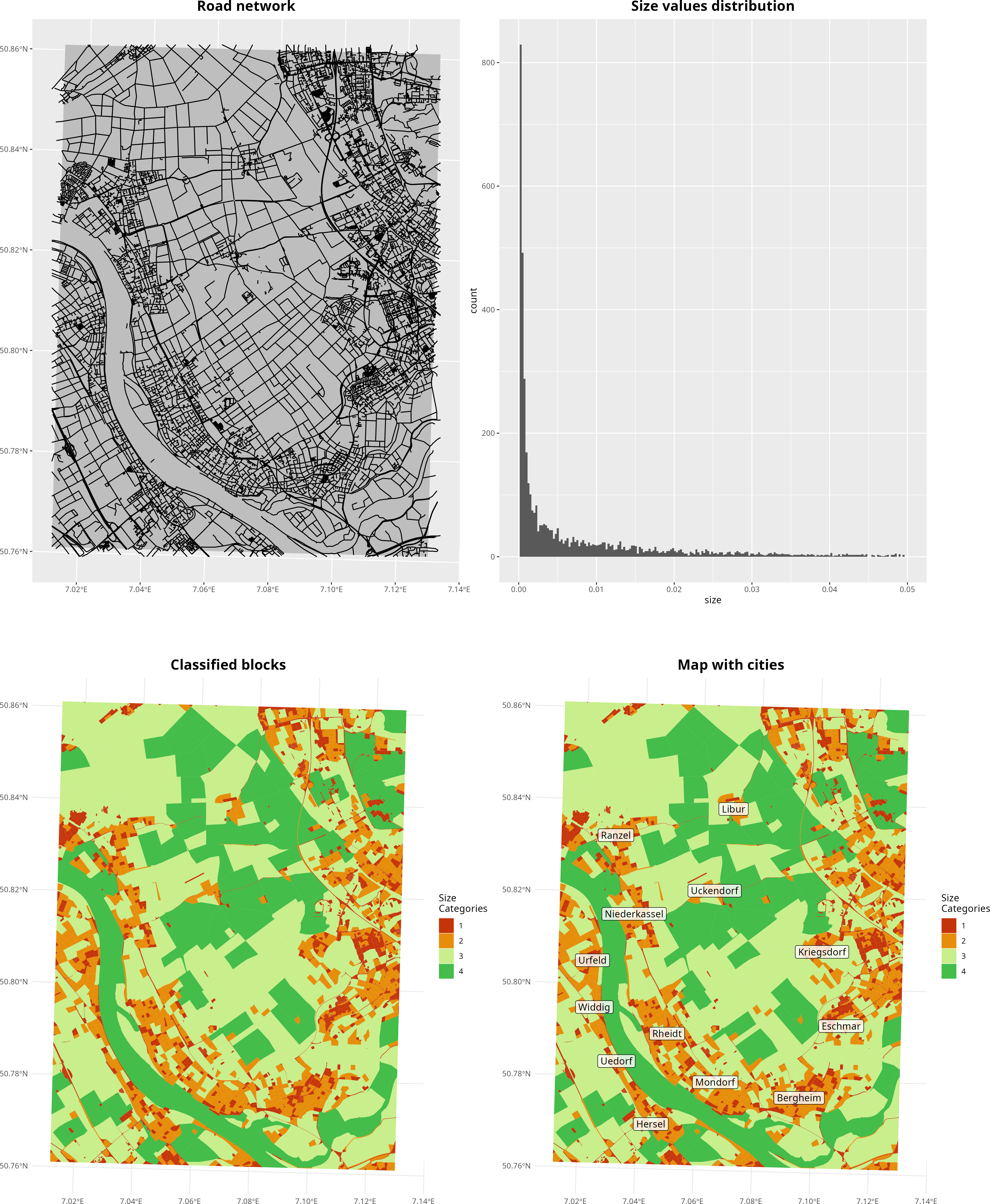
The making of map 8. The process begins with exploring the raw data downloaded from OpenSteetMap. The roads are used to split the background into polygons, and the distribution of size values is examined. Finally, the results are displayed and cities are added to validate the results.
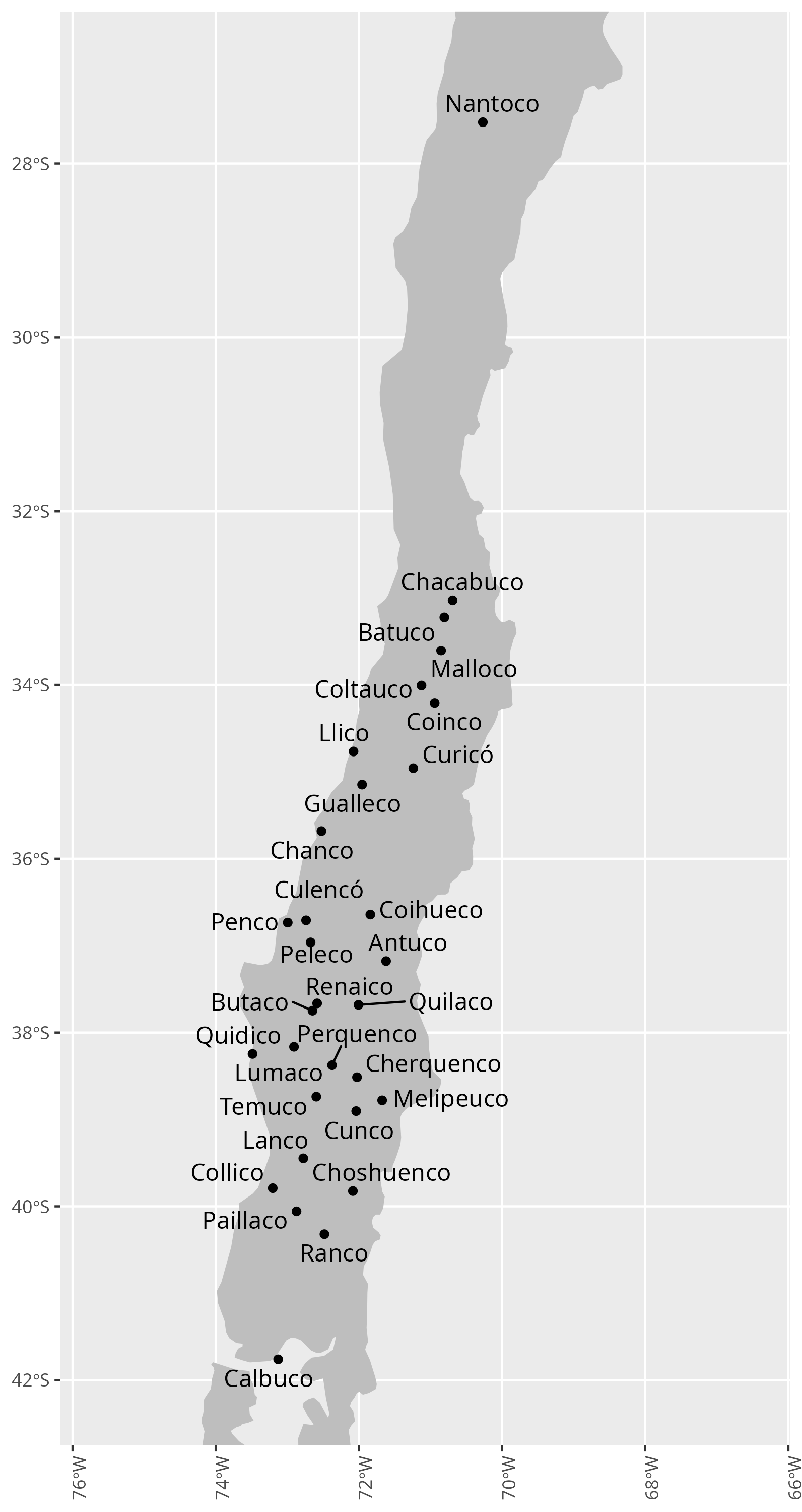
Day 24 – Places and their names
Focus on toponymy (place names). Experiment with font choices, label placement, typography, multiple languages, or the history and meaning behind a name.
In Mapudungun, the language of the Mapuche people, ko means water. As a suffix in Chilean toponymy, it is related to streams or wetlands. Here is a preliminary collection of such names. Note that the outlier Nantoco was named by Mapuches who migrated to this place as mineworkers.
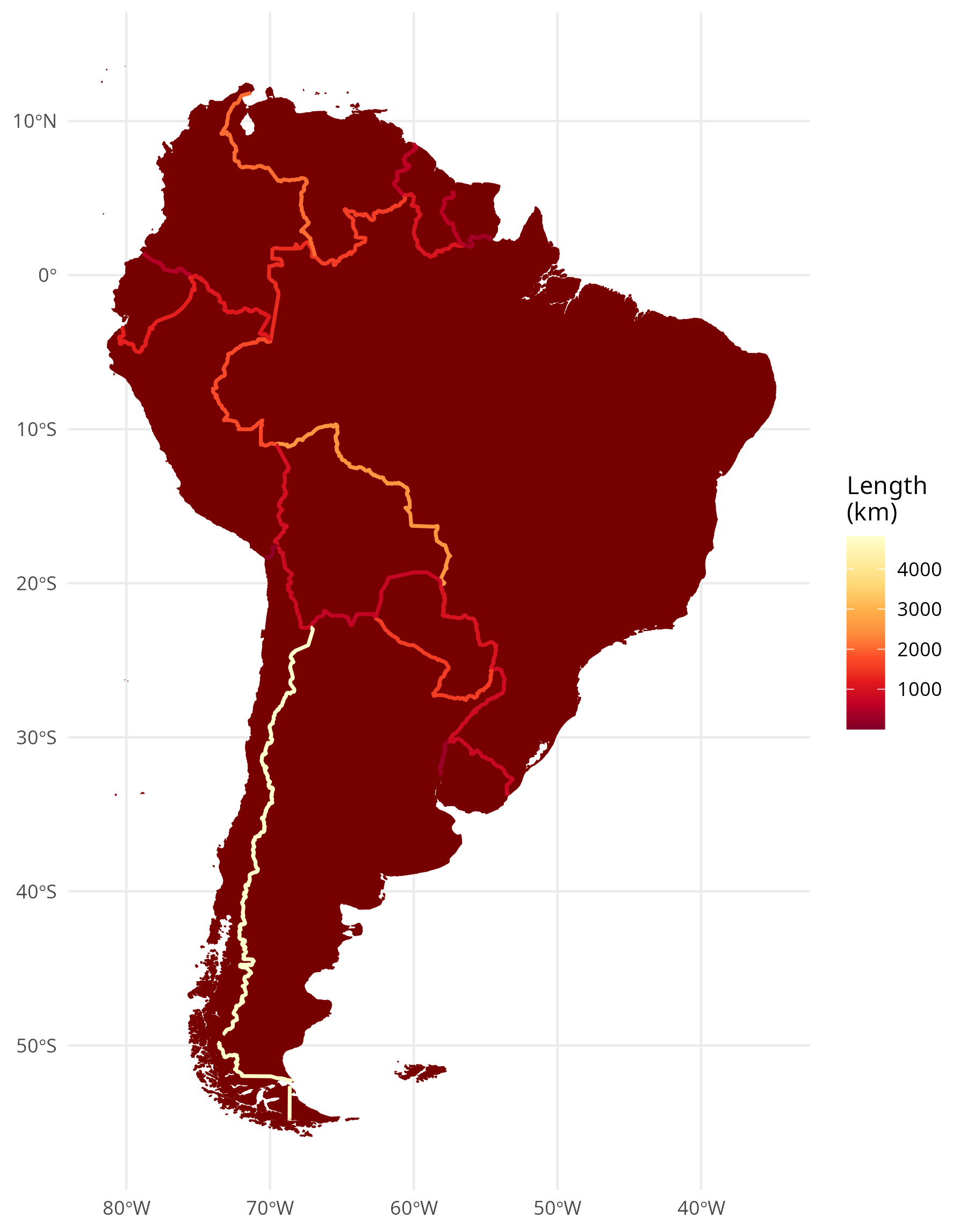
Day 27 – Boundaries
Map lines of division—political, physical, ecological, or conceptual. Explore the meaning and impact of a dividing line, real or perceived.
Borderlines between South American countries. Coloured according to their extent.
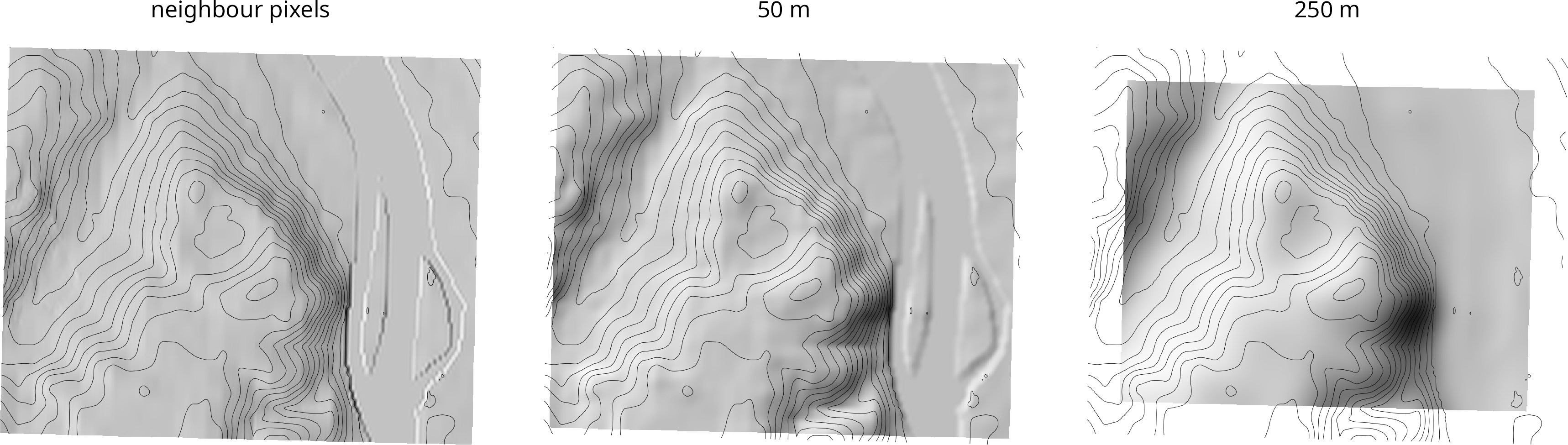
Day 29 – Raster
Challenge Classic: Map using raster data. Focus on satellite imagery, elevation models (DEMs), land cover, or pixel-based art.
The Rodderberg, located on the opposite side of the Rhine River from the Siebengebirge, is an inactive volcano. Although its last eruption was 250,000 years ago, the crater can still be seen in the landscape today. Here, I used my own procedure to contrast the elevations of the south-east and north-west quarters of a circular window. I modified the radius and compared the results with those obtained using the standard procedure of considering only the eight neighbouring pixels in a DEM.
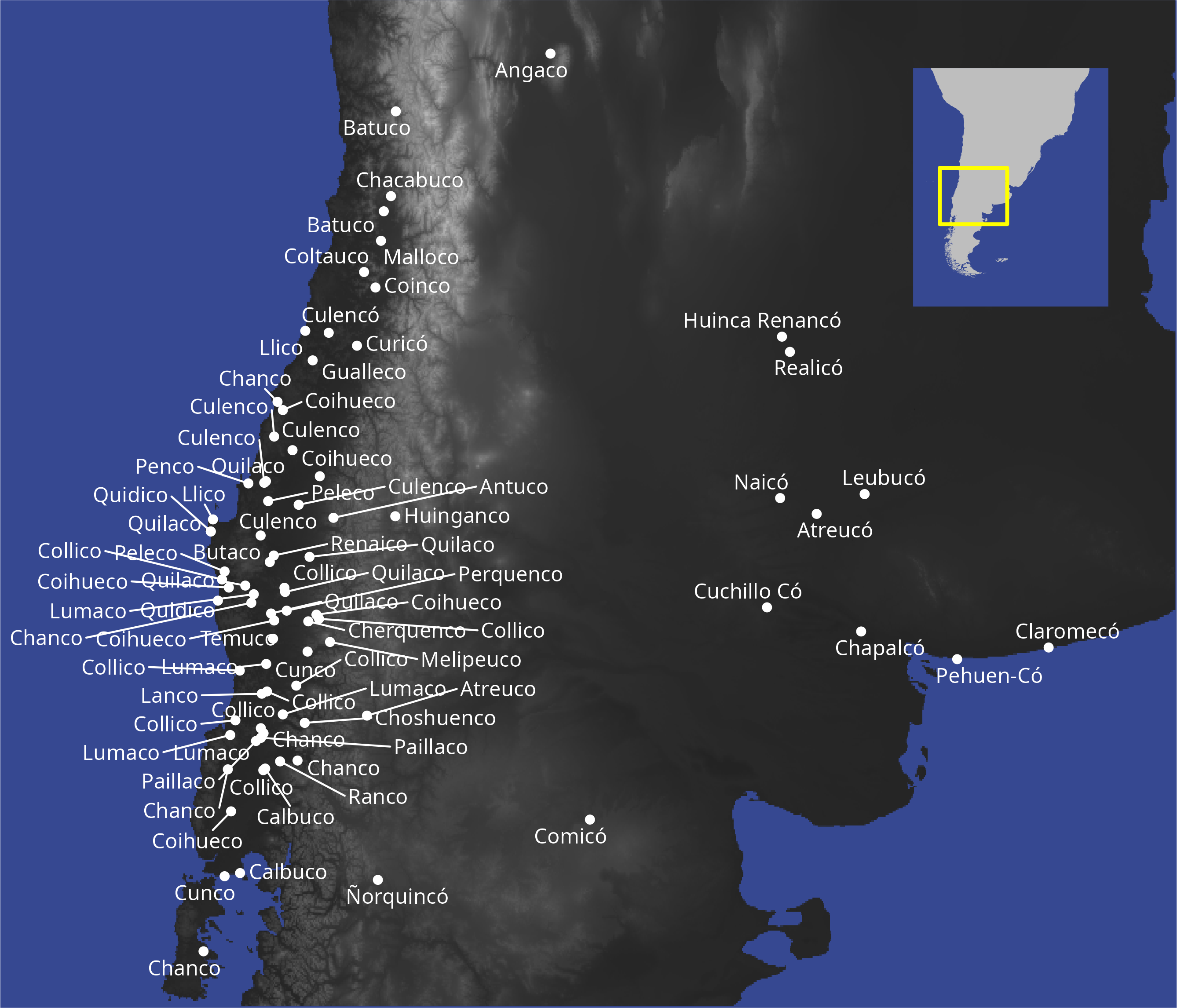
Day 30 – Makeover
Take a map you made during the month or an older piece and redesign it. Focus on improving the aesthetics, clarity, or data communication.
This is not the final version, but an improvement on map 24. I added multiple name occurrences in Chile and expanded the map to include the Argentinean side, showing almost all toponyms, including the Mapudungún word ko for water.