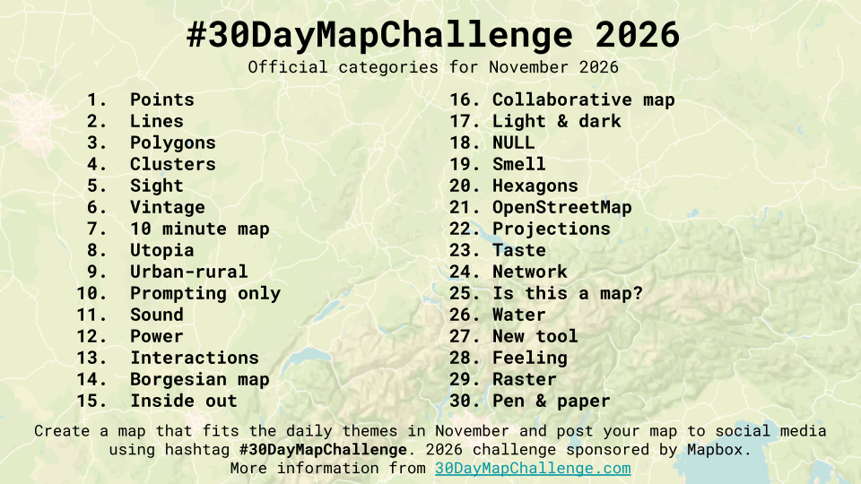
#30DayMapChallenge 2026

R
GIS
cartography

Here’s another round of daily maps. What’s the philosophy this year? Less is more.

Author
Published

November 1, 2026

Another attempt to fulfill the #30DayMapChallenge.

This year I will focus my work using ggplots for the graphics and applying minimalistic layouts. Yo may also find inspiration in further contributions (see one of those ).

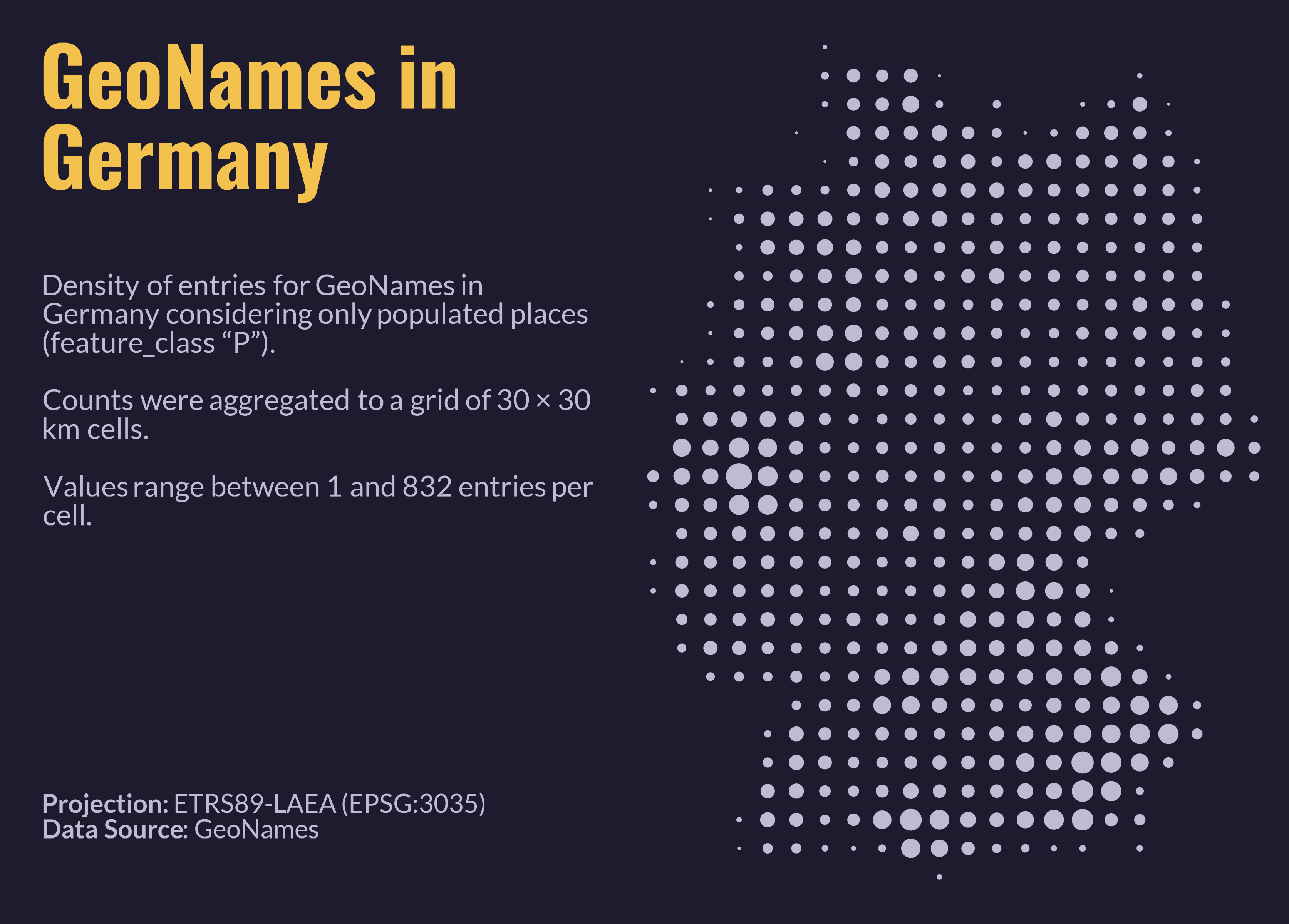
Day 4 – Clusters

Clusters of something. Hotspots, groups, things that gather together.

Show R code
# Load libraries
library(readr)
library(dplyr)
library(sf)
library(ggplot2)
library(ggtext)
library(patchwork)
library(showtext)

# Load geonames for Germany
temp <- tempfile(fileext = ".zip")
download.file(
  url = "https://download.geonames.org/export/dump/DE.zip",
  destfile = temp,
  mode = "wb")

# Name columns in data set
cols <- c(
  "geonameid", "name", "asciiname", "alternatenames", "latitude", "longitude",
  "feature_class", "feature_code", "country_code", "cc2", "admin1_code",
  "admin2_code", "admin3_code", "admin4_code", "population", "elevation", "dem",
  "timezone", "modification_date"
)

# Import data set and transform to spatial features
DE <- read_tsv(
  unz(temp, "DE.txt"),
  col_names = cols,
  quote = "",
  na = "",
  col_types = cols(
    .default = col_character(),
    geonameid = col_integer(),
    latitude = col_double(),
    longitude = col_double(),
    population = col_double(),
    elevation = col_integer(),
    dem = col_integer(),
    modification_date = col_date()
  )
) |> 
  filter(feature_class == "P") |> # Only populated areas
  st_as_sf(coords = c("longitude", "latitude"), crs = st_crs(4326)) |> 
  st_transform(crs = st_crs(3035)) # Transform to EPSG:3035 (LAEA Europe))

# Create a grid of 10 by 10 km
bbox <- st_bbox(DE)

tile_size = 30000
DE_grid = st_bbox(
  c(
    xmin = floor(bbox[["xmin"]] / tile_size),
    ymin = floor(bbox[["ymin"]] / tile_size),
    xmax = ceiling(bbox[["xmax"]] / tile_size),
    ymax = ceiling(bbox[["ymax"]] / tile_size)
  ) * tile_size,
  crs = st_crs(3035)
) |> 
  st_as_sfc() |> 
  st_make_grid(
    cellsize = tile_size,
    what = "polygons",
    square = TRUE
  ) |> 
  st_sf(geometry = _)

DE_grid$cell_id <- seq_len(nrow(DE_grid))

# Count geonames per grid cell
DE_density <- DE_grid |> 
  mutate(n_geonames = lengths(st_intersects(DE_grid, DE))) |> 
  st_centroid() |> 
  filter(n_geonames > 0)

# The plot ---------------------------------------------------------------------

# Selecting colors
bg_col    <- "#1f1b2e"
title_col <- "#f2c14e"
text_col  <- "#c0bbd3"

# Selecting fonts
font_add_google("Oswald", "title_font")
font_add_google("Lato", "body_font")
showtext_auto()
showtext_opts(dpi = 300)

# Map only
the_map <- DE_density |>
  ggplot() +
  geom_sf(
    mapping = aes(size = n_geonames),
    shape = 19,
    colour = text_col
  ) +
  scale_size_area(
    max_size = 7,
    guide = "none"
  ) +
  coord_sf(
    crs = 3035,
    datum = NA,
    expand = FALSE, clip = "off") + # datum = NA removes graticule/axes
  theme_void(base_size = 12)

# helper: one text block, anchored at the top-left of its own panel
text_block <- function(label, family, size_pt, colour) {
  ggplot(tibble(x = 0, y = 1, label = label)) +
    geom_textbox(
      aes(x = x, y = y, label = label),
      hjust = 0, vjust = 1,
      width = unit(1, "npc"),
      box.colour = NA, fill = NA,
      box.padding = unit(rep(0, 4), "pt"),
      box.margin  = unit(rep(0, 4), "pt"),
      colour = colour, family = family,
      size = size_pt / .pt,  # geom_textbox size is in mm, so convert from pt
      lineheight = 1
    ) +
    coord_cartesian(
      xlim = c(0, 1),
      ylim = c(0, 1),
      expand = FALSE,
      clip = "off") +
    theme_void()
}

the_title <- text_block(
  "**GeoNames in Germany**",
  "title_font", 50, title_col
)

the_subtitle <- text_block(
  sprintf(
    paste(
      "Density of entries for GeoNames in Germany considering only populated",
      "places (feature_class \"P\").<br><br>",
      "Counts were aggregated to a grid of %d × %d km cells.<br><br>",
      "Values range between %d and %d entries per cell."
    ),
    tile_size / 1000, tile_size / 1000, min(DE_density$n_geonames),
    max(DE_density$n_geonames)
  ),
  "body_font", 18, text_col
)

the_caption <- text_block(
  "**Projection:** ETRS89-LAEA (EPSG:3035)<br>**Data Source**: GeoNames",
  "body_font", 16, text_col
)

# stack: fixed heights in inches, the spacer absorbs the remaining space
the_side <- the_title / the_subtitle / the_caption / plot_spacer() +
  plot_layout(heights = unit(c(2.0, 4.5, 0.5, 1), c("in", "in", "in", "null")))

fig_h <- 8
margin_in <- 0.3
side_w <- 5                     # text column width in inches

bb    <- st_bbox(DE_density)
asp   <- unname((bb["xmax"] - bb["xmin"]) / (bb["ymax"] - bb["ymin"]))
map_w <- asp * (fig_h - 2 * margin_in)
gap_w <- 0.2    # separation between text and map, in inches

fig_w <- side_w + gap_w + map_w + 2 * margin_in

finalPlot <- (the_side | plot_spacer() | the_map) +
  plot_layout(widths = c(side_w, gap_w, map_w)) +
  plot_annotation(theme = theme(plot.margin = margin(margin_in, margin_in, margin_in, margin_in, "in"))) &
  theme(
    plot.background  = element_rect(fill = bg_col, colour = NA),
    panel.background = element_rect(fill = bg_col, colour = NA)
  )

ggsave("04-clusters.png", finalPlot,
       width = fig_w, height = fig_h, dpi = 300, bg = bg_col)

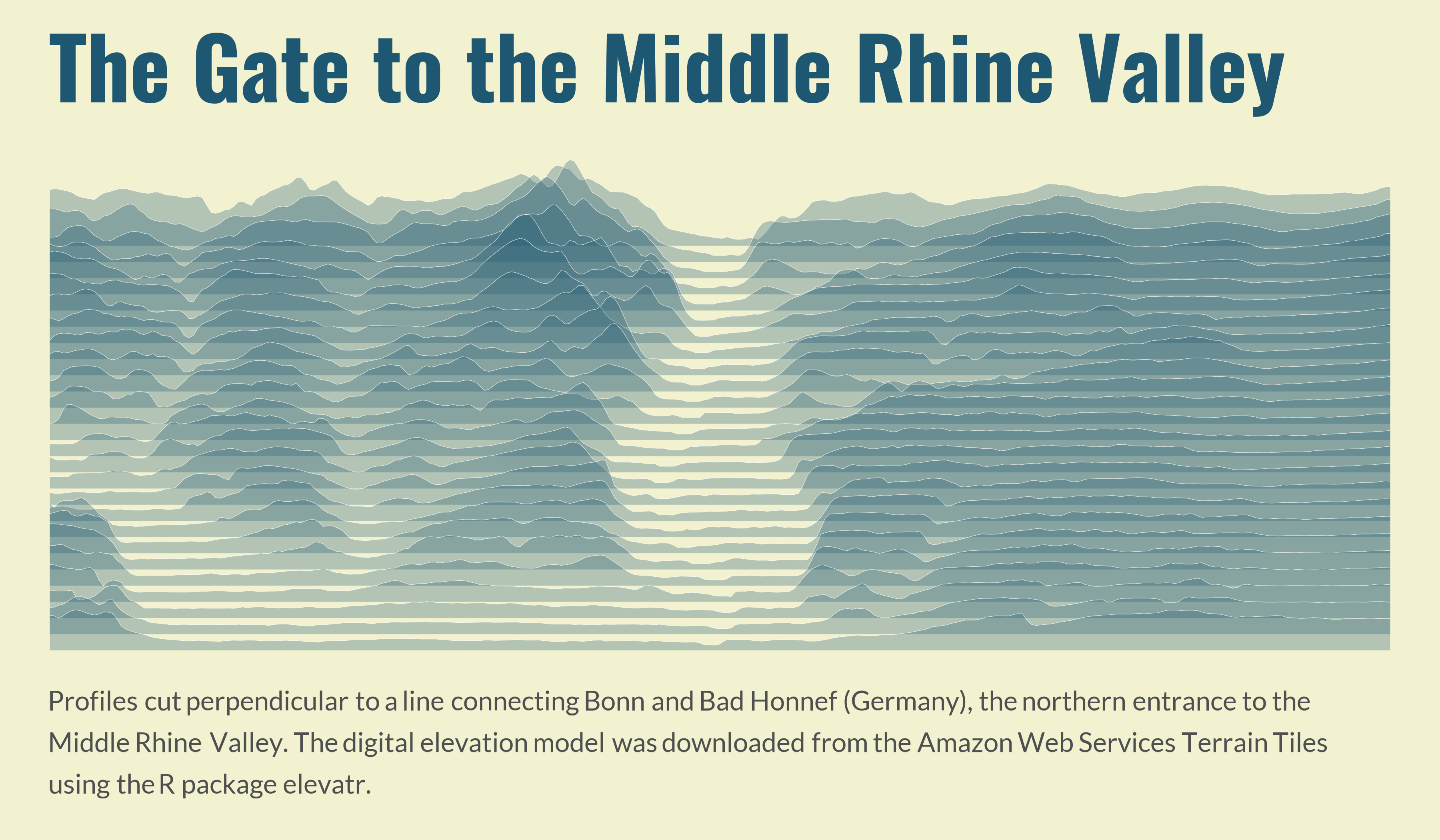
Day 5 – Senses: Sight

How do you see something? Maybe map a viewshed?

Show R code
# Load required packages
library(sf)
library(terra)
library(elevatr)
library(tibble)
library(dplyr)
library(purrr)
library(ggplot2)
library(ggridges)
library(showtext)
library(ggtext)

# Create start-end points
view_axis <- tribble(
  ~fid, ~x, ~y,
  "Bonn", 7.109, 50.736,
  "Bad Honnef", 7.217,  50.642) |> 
  st_as_sf(coords = c("x", "y"), crs = st_crs(4326)) |> 
  st_transform(crs = st_crs(3035)) # Transform to EPSG:3035 (LAEA Europe))

# Extracting coordinates
p1 <- st_coordinates(view_axis)[1, ]
p2 <- st_coordinates(view_axis)[2, ]

d <- 15000 # offset in metres

# unit vector along the axis p1 -> p2
v <- (p2 - p1) / sqrt(sum((p2 - p1)^2))

# unit vector perpendicular to the axis (rotated +90°)
n <- c(-v[["Y"]], v[["X"]])

# four corners: each point shifted to both sides
corners <- rbind(
  p1 + d * n,
  p1 - d * n,
  p2 - d * n,
  p2 + d * n
)

# rectangle for cropping
bbox <- data.frame(
  id = c("p1_left", "p1_right", "p2_right", "p2_left"),
  X = corners[, 1],
  Y = corners[, 2]
  ) |> 
  st_as_sf(coords = c("X", "Y"), crs = st_crs(view_axis)) |> 
  st_combine() |> 
  st_cast("POLYGON") |> 
  st_sf(geometry = _)

# Load DEM
dem <- bbox |>
  st_transform(crs = st_crs(4326)) |> 
  get_elev_raster(locations = _, z = 11, clip = "locations") |> 
  rast() |> 
  project(y = "EPSG:3035")

# Producing segments
n_seg <- 25 # segments along each edge
n_pts <- 300 # points per transect

# Points dividing an edge into n_seg segments (n_seg + 1 points)
t_seq <- seq(0, 1, length.out = n_seg + 1)

interp <- function(a, b, t) {
  cbind(X = a[1] + t * (b[1] - a[1]),
        Y = a[2] + t * (b[2] - a[2]))
}

left  <- interp(corners[1, ], corners[4, ], t_seq)   # p1 -> p4
right <- interp(corners[2, ], corners[3, ], t_seq)   # p2 -> p3

# Transects as saptial lines
transects <- map(
  seq_len(nrow(left)),
  \(i) st_linestring(rbind(left[i, ], right[i, ]))) |>
  st_sfc(crs = st_crs(view_axis)) |>
  st_sf(transect = seq_len(nrow(left)), geometry = _)

# Points from transects
s <- seq(0, 1, length.out = n_pts)

transect_points <- map_dfr(seq_len(nrow(left)), \(i) {
  tibble(
    transect = i,
    point = seq_len(n_pts),
    dist_m = s * sqrt(sum((right[i, ] - left[i, ])^2)),
    X = left[i, "X"] + s * (right[i, "X"] - left[i, "X"]),
    Y = left[i, "Y"] + s * (right[i, "Y"] - left[i, "Y"])
    )
  }) |>
  st_as_sf(coords = c("X", "Y"), crs = st_crs(dem)) |> 
  vect()

# Extract elevation
transect_points$z <- extract(dem, transect_points, method = "bilinear")[, 2]

# Convert to database and fill gaps
transect_df <- transect_points |>
  st_as_sf() |>
  st_drop_geometry() |>
  group_by(transect) |>
  arrange(point, .by_group = TRUE) |>
  mutate(z = approx(dist_m[!is.na(z)], z[!is.na(z)],
    xout = dist_m, rule = 2)$y) |>
  ungroup()

# The plot ---------------------------------------------------------------------

# Colors
bg_col <- "#f2f2d1"
title_col = "#1d5772"
text_col <- "#4f4f4f"

# Loading fonts
font_add_google("Oswald", "title_font")
font_add_google("Lato", "body_font")
showtext_auto()

the_ridges <- transect_df |>
  ggplot() +
  aes(
    x = dist_m,
    y = transect,
    height = z - min(z) + 20,
    group = transect) +
  geom_ridgeline(
    scale = 6 / diff(range(transect_df$z)),
    fill = title_col,
    colour = "white",
    linewidth = 0.1,
    alpha = 0.3
  ) +
  scale_x_continuous(expand = c(0, 0)) + # no padding left and right
  coord_cartesian(clip = "off") + # don't cut the line ends at the panel edge
  labs(
    title = "The Gate to the Middle Rhine Valley",
    caption = paste(
      "Profiles cut perpendicular to a line connecting Bonn and Bad Honnef",
      "(Germany), the northern entrance to the Middle Rhine Valley.",
      "The digital elevation model was downloaded from the",
      "Amazon Web Services Terrain Tiles using the R package elevatr."
    )
  ) +
  theme_void() +
  theme(
    plot.background = element_rect(fill = bg_col, colour = NA),
    plot.margin = margin(20, 30, 20, 30), # top, right, bottom, left (pt)
    plot.title = element_text(
      family = "title_font",
      face = "bold",
      colour = title_col,
      size = 160,
      hjust = 0,
      margin = margin(t = 0, b = 10) # t shifts it down, b = gap to the ridges
    ),
    plot.title.position = "plot", # align to the plot edge, not the panel
    plot.caption = element_textbox_simple(
      family = "body_font",
      colour = text_col,
      size = 50,
      lineheight = 0.5,
      margin = margin(t = 10, b = 5)
    ),
    plot.caption.position = "plot"
  )

# the_ridges

ggsave(
  "05-sight.png", the_ridges,
  width = 12,
  height = 7,
  dpi = 300,
  bg = bg_col)

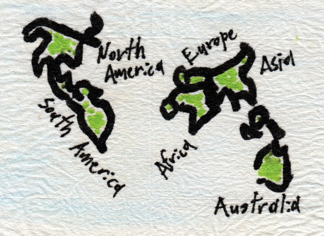
Day 7 – Ten Minute Map

You have no more than 10 minutes to complete this map.

The World in a Tea Bag. I used the Equal Earth projection (really!) as reference and the blind contour drawing technique, working with different markers and pens on upcycled tea bag paper.

Day 8 – Utopia

A map of something which could be.

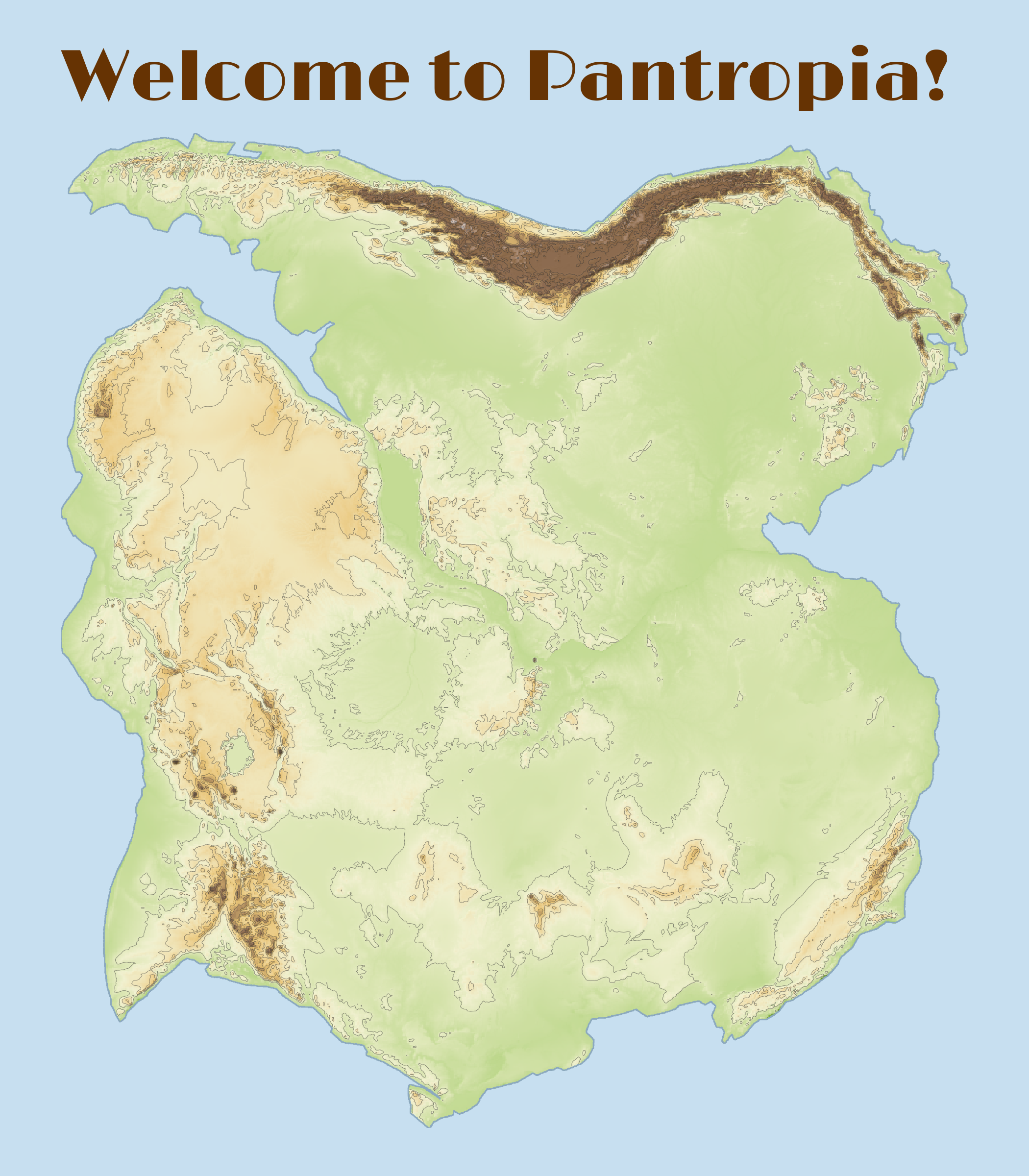
Two sisters meet again in this super-continent.

Show R code
# Fit South America to Africa with a rigid rotation on the sphere
# (shape and area are preserved) and apply the same rotation to a DEM.
# Africa stays fixed; South America is rotated.

# Load packages
library(terra)
library(rnaturalearth)
library(sf)
library(elevatr)
library(ggplot2)
library(tidyterra)
library(ggnewscale)
library(showtext)
library(ggtext)

# 1. Rotation on the sphere (Euler pole + angle, Rodrigues' formula) -----------
to_cart <- function(xy) {                        # lon/lat (deg) -> unit vectors
  lo <- xy[, 1] * pi / 180
  la <- xy[, 2] * pi / 180
  cbind(cos(la) * cos(lo), cos(la) * sin(lo), sin(la))
}

to_lonlat <- function(P) {                       # unit vectors -> lon/lat (deg)
  cbind(atan2(P[, 2], P[, 1]) * 180 / pi,
    asin(pmax(pmin(P[, 3], 1), -1)) * 180 / pi)
}

rot_matrix <- function(pole_lat, pole_lon, angle) {
  k <- to_cart(cbind(pole_lon, pole_lat))[1, ]
  th <- angle * pi / 180
  K <- matrix(c(0, -k[3], k[2],
                k[3], 0, -k[1],
                -k[2], k[1], 0), 3, byrow = TRUE)
  diag(3) + sin(th) * K + (1 - cos(th)) * (K %*% K)
}

rotate_xy <- function(xy, R) to_lonlat(to_cart(xy) %*% t(R))
# inverse rotation: rotate_xy(xy, t(R))

rotate_vect <- function(v, R) {                 # rotate a terra polygon layer
  g <- geom(v)
  xy <- rotate_xy(g[, c("x", "y")], R)
  g[, "x"] <- xy[, 1]
  g[, "y"] <- xy[, 2]
  vect(g, type = "polygons", crs = "EPSG:4326")
}

# 2. Outlines ------------------------------------------------------------------
#    Better than the coastline: the continental-shelf edge, e.g. the 500 m
#    isobath (Bullard et al. 1965), from GEBCO/ETOPO via as.contour().
get_continent <- function(name, d_int = 20000) {
  x <- ne_countries(continent = name, returnclass = "sf")
  v <- aggregate(vect(x)) # dissolve countries into one multipolygon
  parts <- disagg(v) # split into single polygons
  parts <- parts[which.max(expanse(parts)), ] # keep the largest (drops islands)
  return(densify(parts, interval = d_int)) # Densify so that edges are represented by enough vertices
}

sa <- get_continent("South America")
af <- get_continent("Africa")

# Facing margins only (adjust the boxes to your data): east coast of South
# America and west coast of Africa
sa_pts <- crds(as.lines(sa))
sa_pts <- sa_pts[sa_pts[, 1] > -55 & sa_pts[, 2] > -40, ]
af_pts <- crds(as.lines(af))
af_pts <- af_pts[af_pts[, 1] < 15 & af_pts[, 2] > -35 & af_pts[, 2] < 38, ]
A_cart <- to_cart(af_pts)

# 3. Misfit: symmetric mean nearest distance between both margins (km) ---------
#    (small when gaps and overlaps are small)
misfit <- function(par) {
  R <- rot_matrix(par[1], par[2], par[3])
  B <- to_cart(rotate_xy(sa_pts, R))
  S <- B %*% t(A_cart)                          # cosines between all pairs
  d_ab <- sqrt(pmax(2 - 2 * apply(S, 1, max), 0))   # chord lengths (unit sphere)
  d_ba <- sqrt(pmax(2 - 2 * apply(S, 2, max), 0))
  6371 * (mean(d_ab) + mean(d_ba))
}

# Starting values near the classic Bullard et al. (1965) fit (check the sign!)
start <- c(pole_lat = 44, pole_lon = -31, angle = 57)
fit <- optim(start, misfit, method = "Nelder-Mead",
             control = list(maxit = 2000, reltol = 1e-10))
fit$par
fit$value
R <- rot_matrix(fit$par[1], fit$par[2], fit$par[3])

# 4. Check ---------------------------------------------------------------------
sa_rot <- rotate_vect(sa, R)
plot(af, col = "grey80", ext = ext(-80, 60, -45, 45))
plot(sa_rot, col = adjustcolor("red", 0.4), add = TRUE)

# 5. Apply the same rotation to the DEM (inverse mapping, no holes) ------------
#    A lon/lat raster cannot be rotated by changing its extent, so every
#    cell of the new grid is traced back to the original DEM.

# Load DEMs
dem_sa = sa |> 
  st_as_sf() |> 
  get_elev_raster(locations = _, z = 4, clip = "locations") |> 
  rast()

dem_af = af |> 
  st_as_sf() |> 
  get_elev_raster(locations = _, z = 4, clip = "locations") |> 
  rast()

tgt <- rast(ext(sa_rot), resolution = res(dem_sa), crs = "EPSG:4326")
xy_tgt <- xyFromCell(tgt, 1:ncell(tgt))
xy_src <- rotate_xy(xy_tgt, t(R))               # inverse rotation

vals <- extract(dem_sa, xy_src, method = "bilinear")  # "near" for categories
tgt[] <- vals[[ncol(vals)]]
dem_sa_rot <- mask(tgt, sa_rot)                 # keep only the rotated outline

# extent covering both rasters, with Africa's resolution and CRS
ext_all <- union(ext(dem_af), ext(dem_sa_rot))
template <- rast(ext_all, resolution = res(dem_af), crs = crs(dem_af))

af_t <- resample(dem_af, template, method = "bilinear")
sa_t <- resample(dem_sa_rot, template, method = "bilinear")

pantropia <- merge(af_t, sa_t)    # cells where af_t is NA are taken from sa_t

land <- as.polygons(ifel(is.na(pantropia), NA, 1), dissolve = TRUE) |> 
  fillHoles()

inside <- rasterize(land, pantropia, field = 1, background = 0)
pantropia_f <- ifel(is.na(pantropia) & inside == 1, 5, pantropia)

# Check the result
plot(pantropia_f)

# New rotation for final display -----------------------------------------------
rotate_raster <- function(r, angle = 22) {   # angle in degrees, clockwise
  th <- angle * pi / 180
  e  <- ext(r)
  cx <- mean(c(e$xmin, e$xmax)); cy <- mean(c(e$ymin, e$ymax))

  # new extent: bounding box of the rotated corners
  cn <- cbind(c(e$xmin, e$xmax, e$xmax, e$xmin),
              c(e$ymin, e$ymin, e$ymax, e$ymax))
  dx <- cn[, 1] - cx; dy <- cn[, 2] - cy
  xr <- cx + dx * cos(th) + dy * sin(th)
  yr <- cy - dx * sin(th) + dy * cos(th)

  tmpl <- rast(ext(min(xr), max(xr), min(yr), max(yr)),
               resolution = res(r), crs = crs(r))

  # for each new cell, find its source position (inverse rotation)
  xy <- xyFromCell(tmpl, seq_len(ncell(tmpl)))
  dx <- xy[, 1] - cx; dy <- xy[, 2] - cy
  src <- cbind(cx + dx * cos(th) - dy * sin(th),
               cy + dx * sin(th) + dy * cos(th))

  values(tmpl) <- extract(r, src, method = "bilinear")[, 1]
  names(tmpl) <- "elev"
  tmpl
}

island <- rotate_raster(pantropia_f, angle = 150) |> 
  trim()

# Check
plot(island)

# Calculating hill shades
exag <- 5
slope  <- terrain(island * exag, "slope",  unit = "radians")
aspect <- terrain(island * exag, "aspect", unit = "radians")
hill   <- shade(slope, aspect, angle = 40, direction = 315)
names(hill) <- "hill"

# coastline polygon from the valid cells
coast <- as.polygons(ifel(is.na(island), NA, 1), dissolve = TRUE)

# The Plot ---------------------------------------------------------------------

# Colors
bg_col <- "#c7dff0"
title_col = "#663303"
text_col <- "#4f4f4f"
coast_col <- "#8ca9be"

# Loading fonts
font_add_google("Limelight", "title_font")
# font_add_google("Inter", "body_font")
showtext_auto()

the_island <- ggplot() +
  # hillshade (grey)
  geom_spatraster(data = hill, aes(fill = hill), show.legend = FALSE) +
  scale_fill_gradientn(colours = grey.colors(100, start = 0.2, end = 1),
                       na.value = NA, guide = "none") +
  new_scale_fill() +
  # terrain colours on top, semi-transparent so the shading shows through
  geom_spatraster(data = island, aes(fill = elev), alpha = 0.65,
                  show.legend = FALSE) +
  scale_fill_hypso_c(palette = "dem_print", na.value = NA, guide = "none") +
  # scale_fill_hypso_c(palette = "wiki-2.0_hypso", na.value = NA, guide = "none") +
  # scale_fill_hypso_c(palette = "wiki-schwarzwald-cont", na.value = NA, guide = "none") +
  # scale_fill_whitebox_c(palette = "atlas", na.value = NA, guide = "none") +
  
  # contours
  geom_spatraster_contour(
    data = island,
    breaks = seq(0, 6000, by = 500)[-1],
    colour = "grey20", linewidth = 0.1, alpha = 0.6
  ) +
  # coastline
  geom_spatvector(data = coast, fill = NA, colour = coast_col, linewidth = 0.3) +
  coord_sf(expand = FALSE, datum = NA) +
  labs(title = "Welcome to Pantropia!") +
  theme_void() +
  theme(
    plot.background = element_rect(fill = bg_col, colour = NA),
    plot.margin = margin(20, 30, 20, 30), # top, right, bottom, left (pt)
    plot.title = element_text(
      family = "title_font",
      face = "bold",
      colour = title_col,
      size = 110,
      hjust = 0,
      margin = margin(t = 0, b = 10) # t shifts it down, b = gap to the ridges
    ),
    plot.title.position = "plot" # align to the plot edge, not the panel
  )

ggsave(
  "08-utopia.png", the_island,
  width = 7,
  height = 8,
  dpi = 300,
  bg = bg_col)
10-11-2026 | Prompting only | |

Map of internet accessibility in Germany. All delivered in a Script for ggmap.

Day 10 – Prompting Only

For this map, make AI work for its money and produce something from start to finish in a chat window or on the command line.

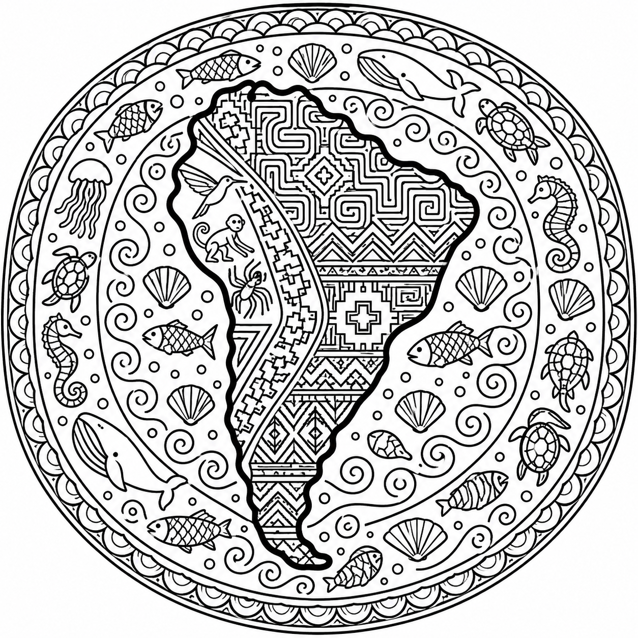
I made something for children (and adults too): a mandala map. The image was created with ChatGPT, using a prompt that Claude helped improve. Feel free to colour it in!

Show Prompt Text
Black-and-white line art in the style of an adult coloring-book page: an
island map of South America, designed as a mandala.

COMPOSITION
- Square format, circular overall composition, centered on a white background.
- South America is shown as an isolated landmass in accurate, recognizable
  proportions, with no neighboring countries, no borders and no other
  continents.
- Around the continent, the ocean forms concentric decorative rings that
  radiate outward and end in a round border.

LINE WORK
- Pure black ink on white. No colour, no grey tones, no shading, no gradients,
  no filled black areas.
- The coastline contour is clearly thicker (about three times) than all
  pattern lines. The inner patterns use fine, evenly weighted lines with
  clear, closed shapes that are easy to colour in.

PATTERNS INSIDE THE CONTINENT (inspired by South American cultures, no
Oriental or Arabic ornaments)
- Andes: stepped Inca and Tiwanaku motifs, chakana crosses, zigzags.
- Amazon basin: dense angular labyrinth patterns inspired by Shipibo-Konibo
  designs.
- Southern region: geometric motifs inspired by Mapuche textiles.
- Coastal desert in the west: stylized animal figures inspired by the
  Nazca lines (hummingbird, monkey, spider).

PATTERNS IN THE OCEAN
- Inner ring: stylized waves and spirals.
- Middle rings: fish, whales, sea turtles, shells, seahorses, jellyfish.
- Outer ring: repeating wave and scale borders.

No text, no letters, no signature, no watermark.